Introduction to Hardware Side Channel Attacks: Recovering an AES Key with Differential Power Analysis

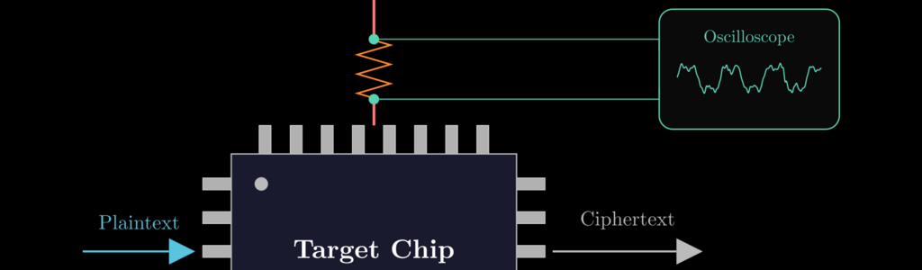
When we review an embedded device, finding a standard crypto algorithm like AES is usually a good sign. It means the vendor is using a well-understood, industry-standard algorithm instead of inventing a new cipher and hoping for the best.

Unfortunately, if the threat model involves the device holding a key secret from an attacker with physical access, securing it becomes a lot harder. Even a strong encryption algorithm implemented correctly can leak information in ways a physical attacker can observe.

There are many ways this leakage can occur, from timing differences in software to electromagnetic emissions from a chip. This post is intended to provide a basic understanding of one such method, in which an attacker records detailed traces of a target device’s power consumption across many cryptographic operations in order to deduce information about the device’s internal state and ultimately recover a secret key.

To demonstrate this, we’ll use a classic side-channel attack to recover an AES-128 key from power measurements taken while a real chip performs encryptions, and visualize the data to build intuition about how the attack works.

All of the traces used below come from the public ChipWhisperer SCA101 course data set. If this post piques your interest, check out the Jupyter notebooks over there. You can work through the lab yourself with or without hardware.

Let’s jump in!

The target

Our target device is a minimal example of crypto performed on hardware using a read-protected key. It takes a plaintext as input and encrypts it with a secret key compiled into the firmware. We’ll act from the perspective of an attacker who does not have any way to extract the firmware, but who does have physical access to the target device.

Our goal is to use this physical access to measure whatever we can about the target during operation and use the information we collect to infer the secret key.

The side channel

Since we cannot attach probes inside the chip itself (well, we could, but it would be very expensive), we’re limited to the pins exposed on the exterior of the chip. All chips consume electricity, and the amount consumed can vary based on the instruction being executed and even based on the data being acted upon. This makes the chip’s power input a natural place to look for information leakage.

A typical setup places a small shunt resistor in the target’s power line and measures the voltage across it. By Ohm’s law, changes in that voltage correspond to changes in the current flowing into the target. Conceptually, the setup looks like this:

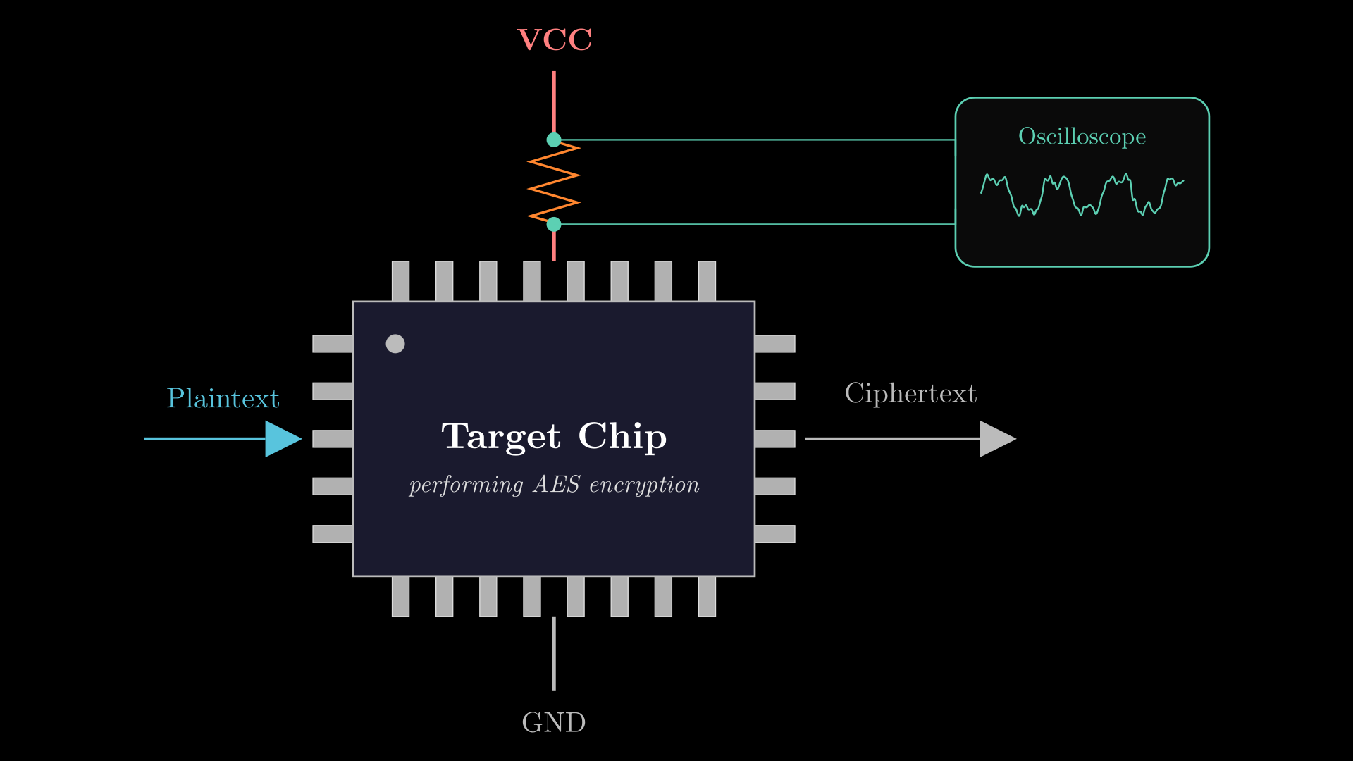
Target chip with oscilloscope probe on power rail

We place the shunt resistor in series with the target chip’s power input, and place our measurement probes on either side of that resistor.

As transistors inside a chip change state, they draw current. The exact amount depends partly on the operation being performed and the data being processed. We can sample this measurement many times per second and build up a full trace across the encryption being performed. Once captured, this trace shows a full timeline of the changes in power consumption across the entire target operation.

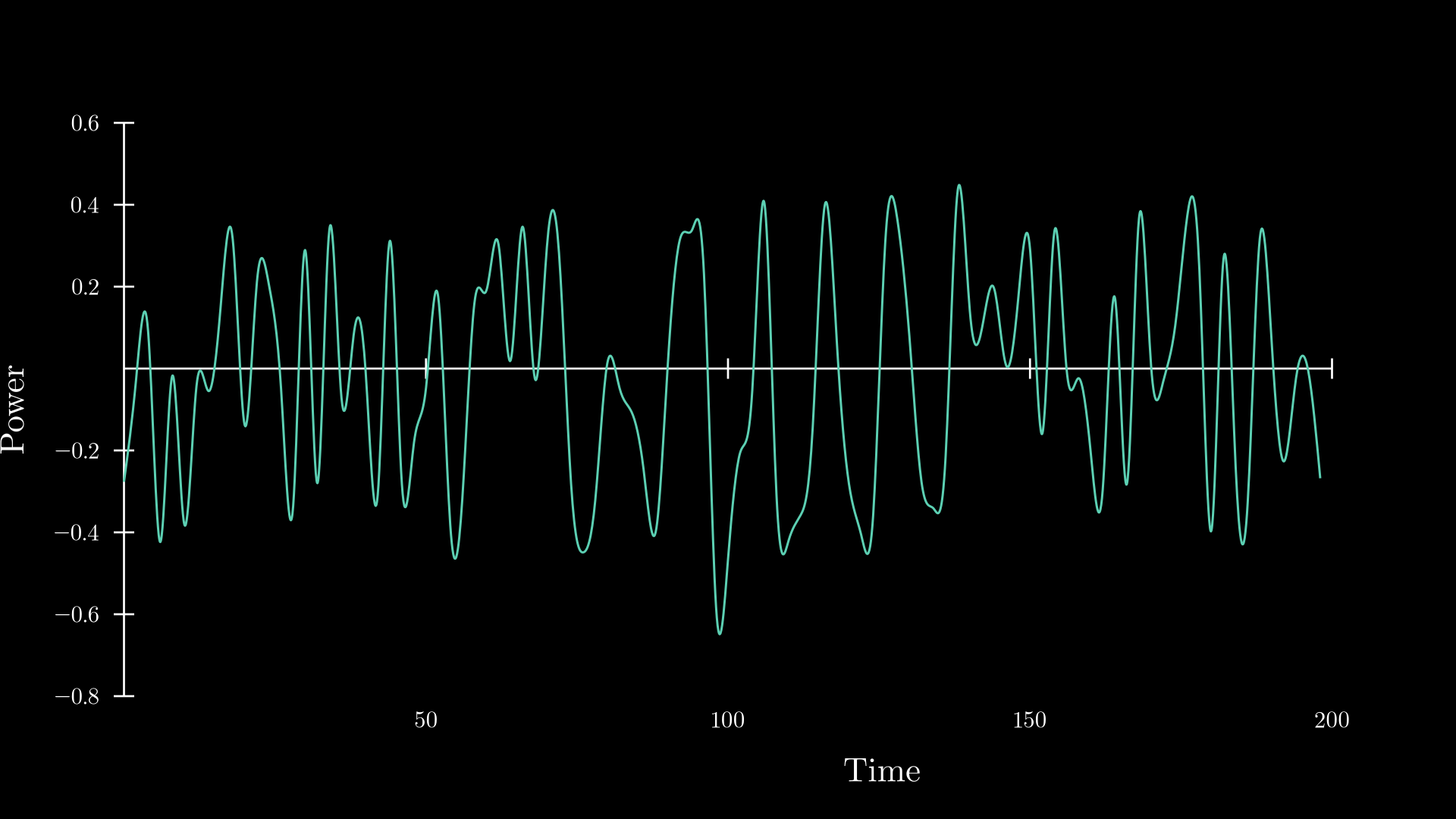
A single power trace: relative power consumption over the course of one AES encryption.

Note: The visualizations in this post are shown at a reduced sample rate to make them easier to look at. The actual traces were recorded at 100x this resolution, and that original sample rate is what the analysis will be performed upon.

This makes a nice looking trace, but the key isn’t exactly jumping out at us. How do we interpret this?

A pile of traces

In this technique, we’ll use a whole collection of traces and analyze them statistically to answer questions about what’s going on in the target. Because we control the plaintext being fed into the device, we can vary it across runs and record what plaintext we fed in each time.

If we stack those captures on top of each other, they look nearly identical:

Most of that shared shape is background activity. The target follows the same execution path and performs the same sequence of AES operations in every trace. What changes is the data passing through those operations.

This is why we vary the plaintext. Different inputs produce different intermediate values, which produce slightly different measurements. Subtracting the average trace makes those variations easier to see, as the animation shows, but we still don’t know which variation is related to our key.

To answer that, we need to choose a value inside AES that we can predict.

Reducing AES to one unknown byte

At the start of AES-128, each plaintext byte is XORed with one byte of the key. The first round’s SubBytes operation then passes the result through the public AES substitution table, or S-Box.

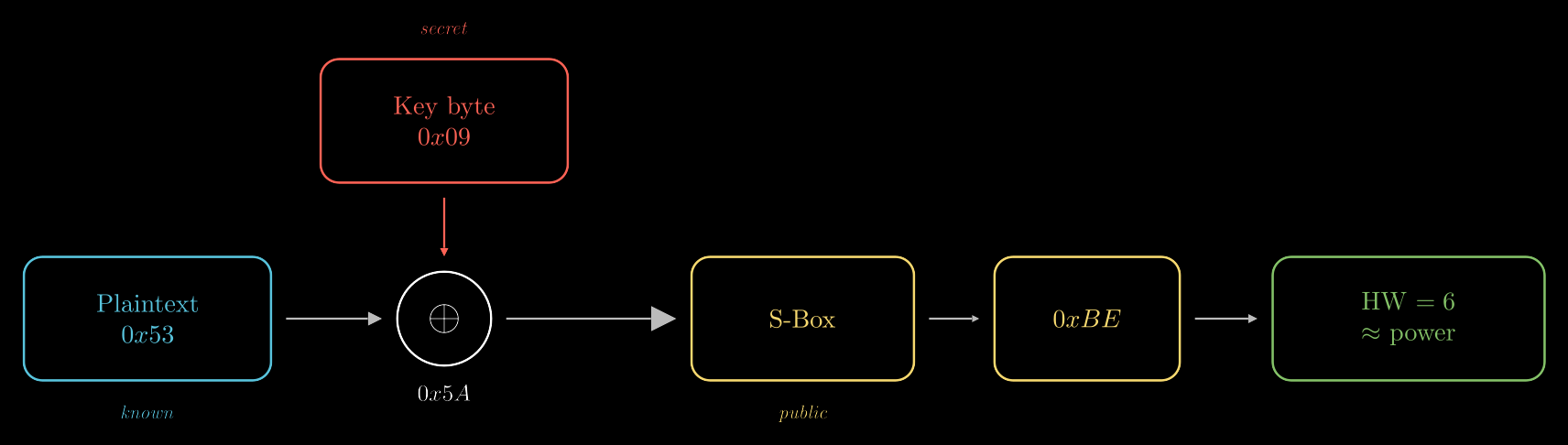
AES Round 1 flow: Plaintext XOR Key byte → S-Box → output byte → Hamming weight ≈ power

For a single byte position, the operation we care about is:

SBox[plaintext_byte XOR key_byte]

We know the plaintext byte. We know the S-Box. The only missing value is one byte of the key, so there are only 256 possibilities to test.

For each possible key byte, we calculate the S-Box output that the device would produce for every captured plaintext. The S-Box is nonlinear, so those 256 key guesses produce distinct sequences of predicted values.

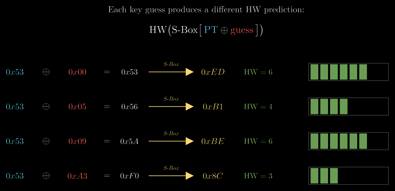
Three key guesses produce three different S-Box outputs and Hamming weights — only the correct guess matches the real power measurements

Of course, the oscilloscope didn’t record a list of S-Box outputs. It recorded voltage. We need one more approximation before we can compare the two.

A (very) rough power model

We know that storing data requires transistors to change state, and that flipping the state of a transistor requires current. From this, we can guess that the amount of power consumed in a given step will correlate roughly with the number of 1 bits to be stored, as more 1 bits likely means more transistors accumulating charge. (The number of 1 bits in a value is called its “Hamming weight”, so we’ll use that term going forward. For example, the Hamming weight of 0b10110100 is four.)

This is all very approximate, and that’s what’s so brilliant about this attack: the model does not need to be very precise at all. The same nonlinearity property that makes AES strong works in our favor here by making small perturbations in the input data magnify into large swings in power draw from trace to trace. As long as our model is good enough to correlate statistically with those swings better than it does with the background noise, we can use it to deduce information.

So if we accept the Hamming weight of a value as a rough proxy for the amount of current needed to store that value, we can start to model the relative amount of power that a chosen instruction should consume for each of our traces.

For every plaintext and key guess, we calculate:

predicted_power = HammingWeight(SBox[plaintext_byte XOR key_guess])

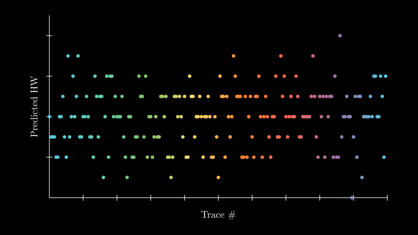
For one candidate key byte, our model gives us one predicted value per trace. The following plot shows the predictions for the 0x09 hypothesis across 200 traces:

Predicted Hamming weight per trace for key guess 0x09

Let the traces rank the guesses

We now calculate the similarity (the Pearson correlation works as a metric here) between our predicted values and the measured values at every sample in the traces.

At most points in time, the chip is doing something unrelated to our target value, so the correlation stays close to zero. Around the point where it handles the first-round S-Box output, the correct key hypothesis should correlate more strongly with the measured power than the incorrect hypotheses.

We repeat this process for all 256 possible key-byte values and compare their strongest correlation peaks. In this data set, 0x09 reaches a peak correlation of 0.86, while the largest incorrect results are approximately 0.25. This tells us two things: 1. The result of the S-Box lookup is most likely stored at the point in time where this peak occurs. 2. The first key byte is most likely 0x09!

Wrong guesses are not guaranteed to produce perfectly flat results. There are all kinds of swings in power consumption outside of the single step we’re modeling that can create incidental peaks. What matters is that the correct candidate is clearly and repeatably separated from the others.

We have now recovered one key byte! Since this first-round operation depends on only one plaintext byte and one key byte, we can repeat the attack independently for each of the 16 byte positions:

for byte_index in range(16):
    for key_guess in range(256):
        predicted = [
            hamming_weight(SBOX[p[byte_index] ^ key_guess])
            for p in plaintexts
        ]
        score[key_guess] = maximum_absolute_correlation(predicted, traces)

    recovered_key[byte_index] = max(score, key=score.get)

Instead of searching the full 2¹²⁸ AES key space, we evaluate at most 16 × 256 = 4,096 key-byte hypotheses. With these clean traces from an unprotected implementation, the analysis itself takes only a few seconds.

Why this belongs in a hardware threat model

The attack requires capabilities that many application threat models reasonably exclude. For this demonstration, an attacker needs enough access to collect aligned measurements while the device performs operations under a stable key. The attacker must also know the corresponding plaintexts. But this is one of the most primitive versions of this attack, chosen because it was easy to illustrate for a blog post. Real, modern attacks leverage machine learning and advanced power modeling to attack more complex algorithms, eliminate the known plaintext requirement, and even infer the machine instructions that make up the target code (SCARE)

Those assumptions are much more realistic for smart cards, embedded devices, self-encrypting drives, hardware roots of trust, accelerators, and other components to which a determined attacker may obtain physical access.

The impact also extends beyond disclosure of one AES key. A device may use long-lived secrets to protect storage, establish its identity, produce attestation evidence, authenticate firmware, or communicate with the rest of a platform. Extracting the right key can undermine the security boundary that the entire system depends on.

This is one reason a hardware security review should begin with the product’s threat model and critical assets rather than a generic checklist. If physical attackers are relevant and a crypto block handles a high-value key, side-channel resistance is something we need to test, not assume.

The OCP S.A.F.E. review framework makes that distinction explicit. Its Scope 1 and Scope 2 reviews cover areas such as firmware, cryptographic construction, key handling, and trust boundaries. Scope 3 adds resilience to physical attacks, including whether cryptographic blocks are designed to resist side-channel analysis and whether critical operations handle glitch attacks securely.

Not every component needs a Scope 3 review. The appropriate depth depends on the assets, deployment environment, and adversary defined in the threat model. A hardware root of trust holding a long-term device identity key, for example, deserves different physical scrutiny from an application processor that never handles the same class of secret.

ivision is an OCP-approved S.A.F.E. Security Review Provider. For us, techniques like the one in this post are one part of a broader device review: understand what the product is expected to protect, map the logical and physical attack surfaces, test the relevant assumptions, and help the vendor address the results before deployment.